
Why a fast model can feel slow: inside the serving queue
Replay a queue and compare fixed batches with continuous admission.
A model can generate tokens quickly once it starts and still make a reader wait. Before useful text appears, the request may pass through admission checks, a queue, prompt processing, and a shared scheduler. A benchmark that measures an already running generation does not describe all of those stages. The user's experience includes time spent waiting for the model to begin.
This article turns one part of that problem into a replayable experiment. Six invented jobs arrive together, each requiring a different number of decoding iterations. You can change how many jobs the server admits at once and compare two rules for filling an empty slot. A second figure lets you inspect the same queue at any point in its execution.
The units are abstract ticks, not milliseconds or measured GPU performance. Each admitted job receives one token of progress per tick, regardless of occupancy. Prompt processing, memory limits, networking, and cancellation overhead are deliberately omitted. Those assumptions make the scheduling effect visible while preventing the figure from masquerading as a prediction of real hardware speed.
Separate waiting from doing the work
Separate the queue from the work
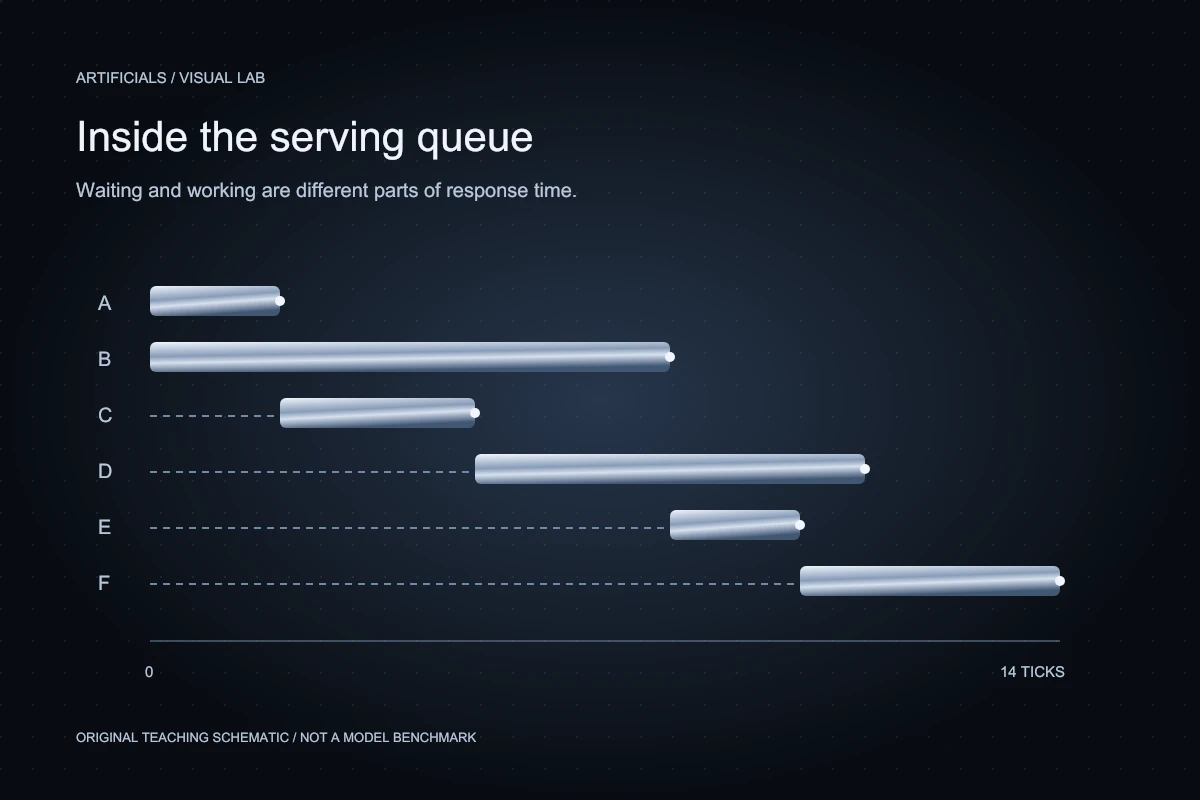
Six jobs arrive at tick zero. Switch the admission rule: dashed segments are waiting; filled segments are service. Both policies share the same time axis at each capacity.
| Job | Wait | Service | Complete |
|---|---|---|---|
| A | 0 | 2 | 2 |
| B | 0 | 8 | 8 |
| C | 2 | 3 | 5 |
| D | 5 | 6 | 11 |
| E | 8 | 2 | 10 |
| F | 10 | 4 | 14 |
Abstract ticks only. First output occurs one tick after service starts. Increasing slots here does not increase per-tick compute cost; real hardware does not have that guarantee.
In the first figure, the empty section before a job starts represents queue waiting. The solid segment represents service: iterations during which that job receives progress. The endpoint marks completion. These quantities answer different questions, so the table reports queue wait and total completion delay separately for every job.
All six jobs arrive at tick zero. Their lengths are two, eight, three, six, two, and four tokens, with a control that can extend the second job to twelve. The scheduler chooses jobs in arrival order, using their identifiers to break the simultaneous-arrival tie. The fixed workload is intentionally small enough that you can trace every slot by hand.
At one slot, both policies behave like a single line: each job waits for the previous job to finish. Increasing slots allows concurrent progress in this model. That is a mathematical property of the fixture, not a promise that doubling a production batch doubles throughput. Real devices can change their per-iteration time as the amount of work changes.
Compare the two admission rules
The fixed-batch rule admits up to the selected capacity, then waits until every admitted job finishes before admitting another group. A short job can finish early while a longer neighbor keeps the batch open. The finished job's slot remains unavailable to the next waiting request under this particular rule, even though that job no longer needs progress.
The continuous rule checks for available slots at each iteration boundary. When a job completes, the next waiting job can occupy its slot on the following iteration. Existing unfinished jobs continue. This reduces idle slot time in the example without changing any job's required number of tokens or claiming that its individual decoding computation became faster.
With two slots, the fixed fixture completes at tick eighteen under the fixed-batch rule and tick fourteen under continuous admission. Those values follow from the stated lengths and equal-cost iterations. They should be read as a worked example, not a speedup claim for a named inference engine or a service-level guarantee.
Follow one short job through the long neighbor
Focus on job C, which needs three tokens. In the fixed two-slot schedule, jobs A and B start together. A finishes after two ticks, but C cannot begin until B finishes at eight. C's short service time does not protect it from waiting behind the longer job's batch boundary.
Under continuous admission, A's slot becomes available at tick two and C enters immediately. B continues in its other slot. C completes at tick five, even though B still has work left. The important change is the opportunity to admit C earlier, not a change in the three units of work that C requires.
Now extend B to twelve tokens. Inspect which rows change and which remain unaffected. This is a useful way to reason about interference: a request's experience can depend on the lengths of other requests sharing its scheduler. An isolated timing test cannot reveal that dependence because there are no neighbors in the experiment.
Replay the queue instead of guessing from an average
Watch a finished job give up its slot
Fixed replay: two slots, continuous admission, lengths 2 / 8 / 3 / 6 / 2 / 4. This figure is independent of the settings above.
Reduced motion is on. Use the slider to explore at your own pace.
0 / 2 tokens · starts 0, finishes 2
0 / 8 tokens · starts 0, finishes 8
0 / 3 tokens · starts 2, finishes 5
0 / 6 tokens · starts 5, finishes 11
0 / 2 tokens · starts 8, finishes 10
0 / 4 tokens · starts 10, finishes 14
Snapshot is taken after admission at each tick boundary. At tick 2, A is completed and C is active with zero tokens. The table in the first figure supplies a static alternative to replay.
The second figure shows waiting, active, and completed jobs at a selected tick under continuous admission with two slots. Scroll downward to advance the replay and upward to reverse it. You can also use the playback controls or move directly to a tick. Each job displays completed tokens against its required length, so progress remains understandable without motion.
At an iteration boundary, a completed job moves to the finished group and an eligible waiting job can become active. The snapshot at tick two therefore already shows C admitted with zero of its three tokens produced. This convention matters: mixing “just before admission” and “just after admission” in different screenshots can create an apparent off-by-one inconsistency.
The replay is a deterministic explanation, not a connection to the site's production traffic. It contains no visitor data, and it does not estimate the load on any API. Its purpose is to make an admission rule inspectable. A useful operational dashboard would need actual request events and a carefully defined clock instead.
Continuous batching is a systems technique, not a free lunch
The Orca research system describes iteration-level scheduling for transformer generation, allowing requests to be managed at a finer granularity than a whole request. That work provides a primary research reference for the scheduling idea. This article's simplified slot model is not an implementation of Orca and does not reproduce its benchmark measurements.
Real serving systems must decide how to divide finite compute and memory among prompt processing and ongoing generation. They may impose token budgets, preempt requests, chunk prompt work, or reserve capacity for different workloads. A configuration that improves completed requests per second can still worsen the waiting time of some requests.
That is why a throughput headline should be accompanied by a workload description and latency distribution. Specify input lengths, output lengths, arrival pattern, concurrency, and the acceptance criteria used to count a request as successful. Without those conditions, comparing two serving numbers can be less informative than the precision of the reported decimals suggests.
First-token time and final-answer time can move differently
A reader notices when useful output first appears, how smoothly it continues, and when the task is complete. These are related but distinct aspects of response time. Streaming can make progress visible sooner without making the final result arrive sooner. A very long output can begin promptly and still take substantial time to finish.
Queue wait contributes before generation begins. Prompt processing adds another cost, especially when the request carries a long context. After generation starts, the gaps between output tokens influence perceived smoothness. A product that reports only an average token rate can hide a long initial wait or a small fraction of requests with disruptive pauses.
The laboratory excludes prompt processing, so its start tick should not be renamed time to first token. Its first generated token appears one tick after service starts. Keeping that convention explicit prevents a teaching simplification from spreading into a misleading production metric. Real instrumentation should name every boundary it measures.
Cache hits solve a different piece of the problem
A reusable prompt prefix may reduce repeated prompt-processing work under a serving system's cache rules. It does not mean that new output tokens no longer require generation. vLLM's automatic prefix caching documentation explicitly distinguishes avoiding repeated prefill work from accelerating the generation of new tokens. That distinction is useful when diagnosing a service that is fast on repeated demonstrations but slow on varied requests.
Measure cold and warm conditions separately. A warm cache can make a narrow test look excellent while a new deployment, changed prompt template, or different user workload behaves otherwise. Cache memory also shares a finite environment with other serving state. A cache policy is part of the capacity plan, not a reason to ignore it.
Our queue fixture has no cache, so none of its gains come from prefix reuse. Keeping that omission explicit lets you identify the one variable it actually explains: admission at iteration boundaries. Combining every optimization into one unlabeled animation would make it harder to know which mechanism caused the result.
Protect the service when demand exceeds capacity
A queue cannot create compute capacity. If requests arrive persistently faster than the system can complete them, waiting grows unless the application changes admission, adds resources, reduces work, or rejects some requests. An unbounded queue can turn a temporary spike into a long period of poor service after the spike has ended.
Define limits around the useful task. Bound input size, output length, simultaneous work, and waiting time. Respect cancellation so abandoned requests do not continue consuming resources without purpose. Decide whether a timed-out request may be retried, and account for the additional load that retries themselves create during an incident.
Fairness also needs a policy. Always prioritizing the shortest jobs may make averages attractive while repeatedly delaying larger legitimate requests. First-come order is easy to explain but may not meet every product requirement. Test the policy against the classes of work the service promises to support, including requests that are expensive but important.
Measure the experience your interface promises
A practical load test should include bursts, quiet periods, long prompts, short outputs, and mixed jobs, with enough detail to reconstruct important failures. Report queue wait, first useful output, completion delay, and rejected or cancelled work separately. Review slower requests rather than hiding them inside a mean.
Use the figures as a starting point for those questions. Change a long job and observe who waits. Change capacity and inspect the assumptions behind the apparent improvement. Then replace the toy clock with measurements from the actual serving path. A fast model becomes a responsive product only when admission, scheduling, and the surrounding application are designed for the same reader experience.