
What does “nearby” mean? A visual lab for AI vector search
Rotate a vector and change the metric to see why rankings move.
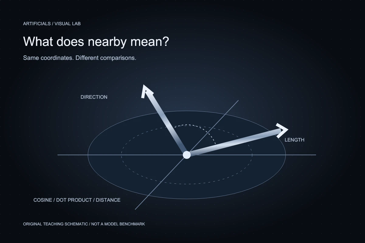
A vector search result can look authoritative because it comes with a precise decimal score. Yet that number is meaningful only after several choices are understood: which representation produced the vectors, which metric compared them, whether their lengths were normalized, and which candidates were allowed into the search. Change one of those choices and “nearest” can mean something different.
This laboratory makes the geometry visible in two dimensions. It does not claim that a real embedding model compresses meaning into a simple compass. The vectors are invented numeric objects, not embeddings of the document labels shown beside them. Their small size lets you inspect every coordinate, check a calculation, and see a ranking change without invoking a remote model.
The first experiment separates direction from length. The second ranks four candidates under three different measures. Together they explain a common source of confusion in AI search: two implementations can process the same vectors correctly and still return different orders because they are answering different mathematical questions.
Rotate direction without hiding length
Direction and length tell different stories
Dashed arrow: query (1, 0). Solid arrow: your candidate. The dotted unit circle marks length one. Every value below is calculated from these coordinates.
Candidate coordinates: (1.311, 0.918). Negative cosine is possible; it is not a negative relevance percentage.
The reference query in the first figure points along the positive horizontal axis and has length one. A second arrow has an adjustable angle and length. Rotate it while watching cosine similarity, dot product, and Euclidean distance. Then leave the angle fixed and stretch it. Different measures respond to those two operations in different ways.
Cosine similarity divides the dot product by the product of the vector lengths. For nonzero vectors, this removes their magnitudes from the comparison and leaves a measure of directional alignment. In this two-dimensional construction, its value is the cosine of the angle between the arrows. A parallel arrow has similarity one; a perpendicular arrow has similarity zero.
Dot product keeps magnitude in the calculation. With the reference fixed at unit length, stretching an aligned candidate increases the dot product. Euclidean distance measures the straight-line separation of the endpoints. A candidate can point in exactly the same direction as the query yet be farther away because its endpoint lies well beyond it.
Work through a case where the measures disagree
Set the candidate angle to zero and its length to two. The query endpoint is at one, zero; the candidate endpoint is at two, zero. Their cosine similarity is one, their dot product is two, and their Euclidean distance is one. All three results are correct. They express different relationships between the same pair of vectors.
Now shorten that candidate until its length is one. The cosine value stays one, the dot product becomes one, and the distance becomes zero. This change did not make the direction more aligned. It brought the endpoints together. Understanding that distinction is more useful than trying to memorize which metric is supposedly best for every search system.
Try ninety degrees next. Cosine and dot product both become zero in the ideal calculation, even though the arrow still has a nonzero length. The endpoints remain separated. At one hundred eighty degrees, the arrows oppose each other and cosine reaches minus one. Floating-point calculations may show tiny residuals near theoretically exact values; display rounding is not a new semantic interpretation.
Normalization changes the comparison contract
L2 normalization divides a nonzero vector by its length, placing its endpoint on a unit sphere. In this two-dimensional view the sphere becomes a circle. After both query and candidates are normalized, their dot products equal their cosine similarities. Squared Euclidean distance is then two minus twice the cosine, so descending cosine and ascending distance produce the same ordering.
That equivalence depends on the normalization condition. Applying it to raw vectors with different lengths can silently change the ranking. A system that was trained to use a particular similarity function should not be switched to another simply because the names sound related. The representation and the comparison rule form a pair.
The scikit-learn metric documentation defines cosine similarity through the normalized dot product. Sentence Transformers documents several similarity functions and discusses the relationship between dot product and cosine for normalized embeddings. These references establish the definitions; the examples in this article are independently constructed teaching data, not reproduced evaluation results.
Scikit-learn: Technical documentation
Change the metric and inspect the ranking
Same candidates, a different nearest neighbor
Choose a metric, rotate the query, then normalize the candidates. The query always has unit length. A–D are coordinate identifiers, not document topics.
| Rank / ID | x, y | Score |
|---|---|---|
| 1 / B | 1.00, 0.00 | 1.000 |
| 2 / A | 2.00, 0.20 | 0.995 |
| 3 / C | 0.20, 0.98 | 0.200 |
| 4 / D | -0.50, 0.80 | -0.530 |
Scores are not interchangeable across metrics. Ties keep the fixture's A–D order. Cosine is undefined for zero vectors, which this experiment excludes.
The second figure starts with four synthetic candidates. Candidate A is long and close to the query direction. Candidate B is shorter and aligned exactly with the initial query. Candidate C sits near the vertical direction. Candidate D points partly toward negative horizontal coordinates. The displayed table preserves the coordinates so that the ordering can be checked independently of the picture.
At the initial query angle, cosine favors B while dot product favors A. Euclidean distance also favors B in this fixture because its endpoint matches the unit query. Rotate the query and watch the order respond. The bars are unnecessary here: a coordinate plot and explicit metric values show the geometry without turning unlike score scales into apparently interchangeable percentages.
The normalize control changes both the candidate representation used for scoring and the positions drawn on the plane. With normalization enabled, compare the order under all three metrics. Apart from exact ties and numerical precision, the ranking relationship follows the identity described above. This is an algebra check, not evidence that normalized search is superior on your documents.
Do not name invented axes after human concepts
It is tempting to label the horizontal axis “technical” and the vertical axis “creative” because that makes a diagram feel intuitive. For real embeddings, such labels require evidence. Individual dimensions are learned features whose interpretations are not usually supplied by a simple human-readable axis title. An attractive chart can become misleading if its labels imply knowledge the model did not provide.
The laboratory therefore calls the axes x and y. Candidate labels are identifiers, not semantic categories. A real embedding model may use hundreds or thousands of dimensions, and a two-dimensional projection can distort distances or hide relationships. Use projected pictures to explore hypotheses, then check the actual metric in the original representation before making a decision.
The same caution applies to clusters. Nearby points can suggest a group worth investigating, but a cluster does not automatically define a topic, intent, or permission boundary. Human inspection and task-specific labels are still needed. A visualization should help reveal what to test rather than quietly manufacture a ground truth.
A high score is not an answer
Suppose a support search returns a policy document with a high cosine similarity to a question. That score indicates a relationship under the chosen representation and metric. It does not prove that the document is current, that its rule applies to the reader, or that the requested fact appears anywhere in the passage.
For a useful result, inspect relevance alongside scope. A historical policy may share nearly every important term with a current one. A neighboring product plan may describe the same workflow with a different allowance. A search system needs metadata and evidence checks to keep a semantically close but inapplicable passage from becoming an authoritative answer.
There is also no universal threshold such as “anything above 0.8 is correct.” Score distributions depend on the model, the data, and the task. Choose thresholds using labeled examples and the cost of mistakes. Recheck them after changing the encoder or preprocessing; the same number can behave differently in a different embedding space.
Build a retrieval test that preserves the hard cases
Start with realistic questions and identify acceptable passages before looking at model rankings. Include paraphrases, short queries, misspellings, and questions whose answer is absent. Add near misses: an archived policy, a sibling feature, or a similarly named person. These examples test whether the system distinguishes useful evidence from merely related wording.
Measure whether a relevant passage appears within the number of results your application can actually inspect. A top-fifty recall result does not describe a product that reads only the first three passages. Review the ordering as well as presence, because an irrelevant first result can consume context space or mislead a downstream answer generator.
Separate exact scoring quality from index approximation. If exhaustive comparison already retrieves the wrong passage, increasing an approximate index's search effort will not fix the underlying representation. If exact scoring works but approximate search misses the candidate, investigate the index settings and candidate coverage. Each failure deserves a repair at the layer where it occurs.
Treat a new embedding model as a new coordinate system
Vectors produced by different embedding models are not automatically compatible even if they have the same dimensionality. Matching the length of two arrays is not evidence that their coordinates share a meaning. Query and document encoders must belong to a supported pairing, with the required prefixes and normalization behavior preserved.
When migrating a search system, build a separate index for the new representation and compare it on a stable evaluation set. Keep the old path available while checking document coverage and relevance. Mixing freshly encoded queries with incompatible old document vectors can produce plausible-looking scores that have no intended interpretation.
Record the encoder version, text preparation, vector dimension, metric, and normalization policy together. That small contract makes troubleshooting much easier than a folder of unexplained arrays. It also makes the meaning of an index rebuild explicit: you are replacing a representation pipeline, not merely refreshing a cache of numbers.
Bring geometry back to the reader's task
The laboratory's arrows are simple enough to inspect, but the lesson applies to larger systems. Similarity is defined by a representation and a metric, and relevance is defined by a user's task. Neither a precise decimal nor an elegant plot removes the need to connect the two.
Use the controls to develop an intuition for direction, magnitude, and distance. Then return to actual passages and ask whether the retrieved evidence answers the question under the right conditions. A good vector search system makes that connection measurable and reviewable, instead of asking the reader to trust whatever happens to be nearby.